This package can be used to support the transformation of datasets
from the storage data format used by IDDO to analysis datasets. The
package is intended for epidemiologists, statisticians and data
scientists with a diverse range of programming ability, but with some
familiarity with R software. This package intends to minimise the time
spent on data manipulation, whilst also encouraging reproducibility and
increasing the accessibility of the data format used by IDDO. All
functions come with documentation and examples which can be viewed using
the ? command.
Data
Most of the data stored by IDDO uses the study data tabulation model (SDTM) format. SDTM features several datasets each with a specific purpose such as participant demographic information or laboratory test results. These datasets are referred to as domains and each have a two letter code (i.e. DM - demographics, MB - microbiology, VS - vital signs).
Within the package, there are several synthetic, example domains that
can be used to gain familiarity with the IDDO-SDTM data. Each domain
starts with the two letter domain code followed by
_RPTESTB.
# demographics (DM) domain
DM_RPTESTB
#> # A tibble: 3 × 22
#>   STUDYID DOMAIN USUBJID SUBJID RFSTDTC DTHDTC DTHFL SITEID INVID INVNAM BRTHDTC
#>   <chr>   <chr>  <chr>    <dbl> <chr>   <chr>  <chr> <chr>  <lgl> <lgl>  <lgl>
#> 1 RPTESTB DM     RPTEST…      1 2023/01 2023/… Y     OXFORD NA    NA     NA
#> 2 RPTESTB DM     RPTEST…      2 2023/01 NA     NA    OXFORD NA    NA     NA
#> 3 RPTESTB DM     RPTEST…      3 2023/02 NA     NA    OXFORD NA    NA     NA
#> # ℹ 11 more variables: AGE <dbl>, AGETXT <lgl>, AGEU <chr>, SEX <chr>,
#> #   RACE <chr>, ETHNIC <chr>, ARMCD <chr>, ARM <chr>, COUNTRY <chr>,
#> #   DMDTC <chr>, DMDY <dbl>

# microbiology (MB) domain
MB_RPTESTB
#> # A tibble: 14 × 39
#>    STUDYID DOMAIN USUBJID     MBSEQ MBGRPID MBREFID MBTESTCD MBTEST     MBMODIFY
#>    <chr>   <chr>  <chr>       <dbl> <lgl>   <lgl>   <chr>    <chr>      <lgl>
#>  1 RPTESTB MB     RPTESTB_001     1 NA      NA      PFALCIPA Plasmodiu… NA
#>  2 RPTESTB MB     RPTESTB_001     2 NA      NA      PFALCIPA Plasmodiu… NA
#>  3 RPTESTB MB     RPTESTB_001     3 NA      NA      PFALCIPA Plasmodiu… NA
#>  4 RPTESTB MB     RPTESTB_001     4 NA      NA      PFALCIPA Plasmodiu… NA
#>  5 RPTESTB MB     RPTESTB_002     1 NA      NA      PFALCIPA Plasmodiu… NA
#>  6 RPTESTB MB     RPTESTB_002     2 NA      NA      PFALCIPA Plasmodiu… NA
#>  7 RPTESTB MB     RPTESTB_002     3 NA      NA      PFALCIPA Plasmodiu… NA
#>  8 RPTESTB MB     RPTESTB_002     4 NA      NA      PFALCIPA Plasmodiu… NA
#>  9 RPTESTB MB     RPTESTB_002     5 NA      NA      PFALCIPA Plasmodiu… NA
#> 10 RPTESTB MB     RPTESTB_002     6 NA      NA      PFALCIPA Plasmodiu… NA
#> 11 RPTESTB MB     RPTESTB_003     1 NA      NA      PFALCIPA Plasmodiu… NA
#> 12 RPTESTB MB     RPTESTB_003     2 NA      NA      PFALCIPA Plasmodiu… NA
#> 13 RPTESTB MB     RPTESTB_003     3 NA      NA      PFALCIPA Plasmodiu… NA
#> 14 RPTESTB MB     RPTESTB_003     4 NA      NA      PFALCIPA Plasmodiu… NA
#> # ℹ 30 more variables: MBTSTDTL <chr>, MBCAT <lgl>, MBORRES <dbl>,
#> #   MBORRESU <chr>, MBSTRESC <dbl>, MBSTRESN <dbl>, MBSTRESU <chr>,
#> #   MBSTAT <lgl>, MBREASND <lgl>, MBNAM <lgl>, MBSPEC <chr>, MBSPCCND <lgl>,
#> #   MBLOC <chr>, MBMETHOD <chr>, VISITNUM <dbl>, VISIT <chr>, VISITDY <dbl>,
#> #   EPOCH <chr>, MBDTC <chr>, MBDY <dbl>, MBTPT <lgl>, MBTPTNUM <lgl>,
#> #   MBELTM <lgl>, MBTPTREF <lgl>, MBSTRF <lgl>, MBEVINTX <lgl>, MBSTRTPT <lgl>,
#> #   MBSTTPT <lgl>, MBCDSTDY <lgl>, MBRPOC <lgl>
DM_RPTESTB contains demographic information such as age,
sex and study treatment arm; there is one row per participant. Whereas,
MB_RPTESTB shows each microbiology test result from the
study with multiple rows per person, per day. SDTM domains, such as the
MB domain, can have up to 4 columns for the results and a variety of
over 20 timing variables, while this preserves the intricacies in the
trial data, it also creates complexity for analysis.
Functions
prepare_domain()
prepare_domain() takes a single IDDO-SDTM domain,
amalgamates the data so that there is one ‘best choice’ result and
timing variable, then pivots the rows by the best choice time variable
(TIME, TIME_SOURCE), the study id
(STUDYID) and participant number (USUBJID).
The different events/findings/tests then become columns and the dataset
is populated with the associated result, providing a condensed dataset
which is more digestible and can be easily merged with other data.
In prepare_domain(), the first parameter is the domain
data frame followed by the two letter domain code.
prepare_domain(MB_RPTESTB,
               "mb")
#> [1] "The timing variable(s) hierarchy being used in prepare_domain() for the MB domain are: MBDY, MBCDSTDY, VISITDY, EPOCH"
#> [1] "Number of rows where values_fn has been used to pick record in the MB domain: 0"
#> # A tibble: 14 × 5
#>    STUDYID USUBJID     TIME  TIME_SOURCE `PFALCIPA_10^6/L`
#>    <chr>   <chr>       <chr> <chr>       <chr>
#>  1 RPTESTB RPTESTB_001 1     DY          899
#>  2 RPTESTB RPTESTB_001 3     DY          0
#>  3 RPTESTB RPTESTB_001 85    DY          450
#>  4 RPTESTB RPTESTB_001 181   DY          2987
#>  5 RPTESTB RPTESTB_002 1     DY          1056
#>  6 RPTESTB RPTESTB_002 4     DY          48
#>  7 RPTESTB RPTESTB_002 86    DY          0
#>  8 RPTESTB RPTESTB_002 182   DY          0
#>  9 RPTESTB RPTESTB_002 273   DY          0
#> 10 RPTESTB RPTESTB_002 362   DY          0
#> 11 RPTESTB RPTESTB_003 2     DY          989
#> 12 RPTESTB RPTESTB_003 5     DY          0
#> 13 RPTESTB RPTESTB_003 85    DY          167
#> 14 RPTESTB RPTESTB_003 184   DY          0
These best choices follow a hierarchical list of variables, so for a
given row, if the first variable in the hierarchy list is not present,
the second will be used unless that is also empty, and so on. For
example, MBSTRESN (standardised numeric result) is
initially used as the best choice result variable, where rows have an
empty MBSTRESN, MBSTRESC (standardised
character result) will be used. If there are still empty rows,
MBMODIFY (modified original result) and finally
MBORRES (original result from data contributor) will be
used to populate the output.
With the best choice timing variable, there is a default hierarchy,
though users are encouraged to specify the list of timing variables
which are most relevant to the study and objectives they have. For
example, a researcher may only want planned visit days as the timing
variable, so they can specify VISITDY. The
TIME_SOURCE changes compared to the previous example as the
hierarchy has changed.
prepare_domain(MB_RPTESTB,
               "MB",
               timing_variables = "VISITDY")
#> [1] "The timing variable(s) hierarchy being used in prepare_domain() for the MB domain are: VISITDY"
#> [1] "Number of rows where values_fn has been used to pick record in the MB domain: 0"
#> # A tibble: 14 × 5
#>    STUDYID USUBJID     TIME  TIME_SOURCE `PFALCIPA_10^6/L`
#>    <chr>   <chr>       <chr> <chr>       <chr>
#>  1 RPTESTB RPTESTB_001 1     VISITDY     899
#>  2 RPTESTB RPTESTB_001 3     VISITDY     0
#>  3 RPTESTB RPTESTB_001 85    VISITDY     450
#>  4 RPTESTB RPTESTB_001 182   VISITDY     2987
#>  5 RPTESTB RPTESTB_002 1     VISITDY     1056
#>  6 RPTESTB RPTESTB_002 3     VISITDY     48
#>  7 RPTESTB RPTESTB_002 85    VISITDY     0
#>  8 RPTESTB RPTESTB_002 182   VISITDY     0
#>  9 RPTESTB RPTESTB_002 273   VISITDY     0
#> 10 RPTESTB RPTESTB_002 366   VISITDY     0
#> 11 RPTESTB RPTESTB_003 1     VISITDY     989
#> 12 RPTESTB RPTESTB_003 3     VISITDY     0
#> 13 RPTESTB RPTESTB_003 85    VISITDY     167
#> 14 RPTESTB RPTESTB_003 182   VISITDY     0
Additional parameters include subsetting the output on the variables
of interest, by using variables_include to select just
weight and temperature in the VS domain example below:
prepare_domain(VS_RPTESTB,
               "vs",
               variables_include = c("TEMP", "WEIGHT"))
#> [1] "The timing variable(s) hierarchy being used in prepare_domain() for the VS domain are: VSDY, VISITDY, EPOCH"
#> [1] "Number of rows where values_fn has been used to pick record in the VS domain: 0"
#> # A tibble: 9 × 6
#>   STUDYID USUBJID     TIME      TIME_SOURCE TEMP_C WEIGHT_kg
#>   <chr>   <chr>       <chr>     <chr>       <chr>  <chr>
#> 1 RPTESTB RPTESTB_001 1         DY          36.2   60
#> 2 RPTESTB RPTESTB_001 3         DY          37.4   NA
#> 3 RPTESTB RPTESTB_001 42        DY          37.5   NA
#> 4 RPTESTB RPTESTB_002 1         DY          37.5   42
#> 5 RPTESTB RPTESTB_002 4         DY          37.2   NA
#> 6 RPTESTB RPTESTB_002 40        DY          37.9   NA
#> 7 RPTESTB RPTESTB_003 2         DY          37.2   9.6
#> 8 RPTESTB RPTESTB_003 5         DY          37.1   NA
#> 9 RPTESTB RPTESTB_003 FOLLOW UP EPOCH       37.7   NA
The location (LOC) and method (METHOD) of a
test or finding may be required in the analysis dataset.
include_LOC and include_METHOD can be set to
TRUE to include them in the column names of the
test/finding along with the units, (i.e. TEMP_AXILLA_C). If
the location or method is NA, then NA will
appear in the column name (i.e. WEIGHT_NA_kg).
prepare_domain(VS_RPTESTB,
               "vs",
               variables_include = c("TEMP", "WEIGHT"),
               include_LOC = TRUE)
#> [1] "The timing variable(s) hierarchy being used in prepare_domain() for the VS domain are: VSDY, VISITDY, EPOCH"
#> [1] "Number of rows where values_fn has been used to pick record in the VS domain: 0"
#> # A tibble: 9 × 7
#>   STUDYID USUBJID     TIME      TIME_SOURCE TEMP_AXILLA_C TEMP_ORAL_CAVITY_C
#>   <chr>   <chr>       <chr>     <chr>       <chr>         <chr>
#> 1 RPTESTB RPTESTB_001 1         DY          36.2          NA
#> 2 RPTESTB RPTESTB_001 3         DY          37.4          NA
#> 3 RPTESTB RPTESTB_001 42        DY          37.5          NA
#> 4 RPTESTB RPTESTB_002 1         DY          NA            37.5
#> 5 RPTESTB RPTESTB_002 4         DY          NA            37.2
#> 6 RPTESTB RPTESTB_002 40        DY          NA            37.9
#> 7 RPTESTB RPTESTB_003 2         DY          37.2          NA
#> 8 RPTESTB RPTESTB_003 5         DY          37.1          NA
#> 9 RPTESTB RPTESTB_003 FOLLOW UP EPOCH       37.7          NA
#> # ℹ 1 more variable: WEIGHT_NA_kg <chr>
When the function pivots the data, they may be occasions where two
rows for the same test/finding/event have the same STUDYID, USUBJID,
TIME value & TIME_SOURCE, in this scenario, the rows are not
uniquely separable so the first row is taken by default (the
first() function used). This can be changed to another
function using the values_fn parameter. The number of rows
affected will be reported in the console when running
prepare_domain() by default, unless
print_messages is set to FALSE.
Once one domain has been transformed, the consistent keys
(STUDYID, USUBJID, TIME,
TIME_SOURCE) enable easy merging with other prepared
domains, allowing for a customised analysis dataset to be built.
left_join(
  prepare_domain(MB_RPTESTB, "MB",  timing_variables = "VISIT"),
  prepare_domain(VS_RPTESTB, "Vs",  timing_variables = "VISIT", include_LOC = TRUE)
)
#> [1] "The timing variable(s) hierarchy being used in prepare_domain() for the MB domain are: VISIT"
#> [1] "Number of rows where values_fn has been used to pick record in the MB domain: 0"
#> [1] "The timing variable(s) hierarchy being used in prepare_domain() for the VS domain are: VISIT"
#> [1] "Number of rows where values_fn has been used to pick record in the VS domain: 0"
#> Joining with `by = join_by(STUDYID, USUBJID, TIME, TIME_SOURCE)`
#> # A tibble: 14 × 10
#>    STUDYID USUBJID     TIME     TIME_SOURCE `PFALCIPA_10^6/L` `BMI_NA_kg/m2`
#>    <chr>   <chr>       <chr>    <chr>       <chr>             <chr>
#>  1 RPTESTB RPTESTB_001 Day 0    VISIT       899               21.5
#>  2 RPTESTB RPTESTB_001 Day 2    VISIT       0                 NA
#>  3 RPTESTB RPTESTB_001 Week 12  VISIT       450               NA
#>  4 RPTESTB RPTESTB_001 Month 6  VISIT       2987              NA
#>  5 RPTESTB RPTESTB_002 Day 0    VISIT       1056              20.5
#>  6 RPTESTB RPTESTB_002 Day 2    VISIT       48                NA
#>  7 RPTESTB RPTESTB_002 Week 12  VISIT       0                 NA
#>  8 RPTESTB RPTESTB_002 Month 6  VISIT       0                 NA
#>  9 RPTESTB RPTESTB_002 Month 9  VISIT       0                 NA
#> 10 RPTESTB RPTESTB_002 Month 12 VISIT       0                 NA
#> 11 RPTESTB RPTESTB_003 Day 0    VISIT       989               0.01
#> 12 RPTESTB RPTESTB_003 Day 2    VISIT       0                 NA
#> 13 RPTESTB RPTESTB_003 Week 12  VISIT       167               NA
#> 14 RPTESTB RPTESTB_003 Month 6  VISIT       0                 NA
#> # ℹ 4 more variables: HEIGHT_NA_cm <chr>, TEMP_AXILLA_C <chr>,
#> #   TEMP_ORAL_CAVITY_C <chr>, WEIGHT_NA_kg <chr>
Standardised Tables for Analysis
The package also contains functions to create standardised analysis
datasets, these start with create_. These functions use the
prepare_domain() function multiple times to extract
specific variables from the domains they reside in. The choice of which
variables to include are based on subject matter expertise, and we
encourage suggestions to improve current tables or to design new tables.
The purpose of these tables is to provide most of the key information
for an analysis, such as the information typically presented in Table 1
of clinical trials. A key limitation is that these functions cannot
address every need of researchers and neither would it be possible to
make an all-encompassing solution due to the large variability in the
dataset within and across diseases. However, these standardised tables
do provide useful key information with minimal user input, ideal for
those who are not experienced programming users.
create_participant_table() creates a one row per
participant analysis table along with several participant characteristic
variables and baseline test information. World Health Organisation child
growth standards are also derived if age, sex, height and weight are in
the dataset; height for age (HAZ), weight for age
(WAZ) and weight for height (WHZ)
-scores
are calculated for participants under the age of 5, with respective
flags (i.e. HAZ_FLAG) for scores outside a typical
range.
create_participant_table(dm_domain = DM_RPTESTB,
                         rp_domain = RP_RPTESTB,
                         vs_domain = VS_RPTESTB)
#> [1] "The timing variable(s) hierarchy being used in prepare_domain() for the VS domain are: VISITDY, EPOCH"
#> [1] "Number of rows where values_fn has been used to pick record in the VS domain: 0"
#> Joining with `by = join_by(STUDYID, USUBJID)`
#> [1] "The timing variable(s) hierarchy being used in prepare_domain() for the RP domain are: VISITDY, EPOCH"
#> [1] "Number of rows where values_fn has been used to pick record in the RP domain: 0"
#> Joining with `by = join_by(STUDYID, USUBJID)`
#> Joining with `by = join_by(STUDYID, USUBJID, AGE_YEARS, SEX, RFSTDTC, RACE,
#> ETHNIC, ARMCD, COUNTRY, SITEID, DTHFL, `BMI_kg/m2`, HEIGHT_cm, WEIGHT_kg,
#> PREGIND_NA)`
#> # A tibble: 3 × 21
#>   STUDYID USUBJID     AGE_YEARS SEX   RFSTDTC RACE  ETHNIC  ARMCD COUNTRY SITEID
#>   <chr>   <chr>           <dbl> <chr> <chr>   <chr> <chr>   <chr> <chr>   <chr>
#> 1 RPTESTB RPTESTB_001        67 F     2023/01 White British PBO   UK      OXFORD
#> 2 RPTESTB RPTESTB_002        18 F     2023/01 White Irish   TRT   UK      OXFORD
#> 3 RPTESTB RPTESTB_003         4 M     2023/02 White British TRT   UK      OXFORD
#> # ℹ 11 more variables: DTHFL <chr>, `BMI_kg/m2` <chr>, HEIGHT_cm <chr>,
#> #   WEIGHT_kg <chr>, PREGIND_NA <chr>, HAZ <dbl>, HAZ_FLAG <int>, WAZ <dbl>,
#> #   WAZ_FLAG <int>, WHZ <dbl>, WHZ_FLAG <int>
create_malaria_pcr_table() creates a one row per person,
per timepoint table combining the polymerase chain reaction (PCR) test
information, drawing from the Pharmacogenomics Genetics (PF), Disease
Response and Clinical Classification (RS) and (optionally) disposition
(DS) domains.
create_malaria_pcr_table(pf_domain = PF_RPTESTB,
                         rs_domain = RS_RPTESTB)
#> [1] "The timing variable(s) hierarchy being used in prepare_domain() for the PF domain are: PFDY, PFCDSTDY, VISITDY, EPOCH"
#> [1] "Number of rows where values_fn has been used to pick record in the PF domain: 0"
#> [1] "The timing variable(s) hierarchy being used in prepare_domain() for the RS domain are: RSDY, RSCDSTDY, VISITDY, EPOCH"
#> [1] "Number of rows where values_fn has been used to pick record in the RS domain: 0"
#> Joining with `by = join_by(STUDYID, USUBJID, TIME, TIME_SOURCE)`
#> # A tibble: 3 × 6
#>   STUDYID USUBJID     TIME  TIME_SOURCE INTP_NA       WHOMAL01_NA
#>   <chr>   <chr>       <chr> <chr>       <chr>         <chr>
#> 1 RPTESTB RPTESTB_001 46    DY          RECRUDESCENCE LATE PARASITOLOGICAL FAIL…
#> 2 RPTESTB RPTESTB_002 50    DY          INDETERMINATE ACPR
#> 3 RPTESTB RPTESTB_003 43    DY          REINFECTION   ACPR
A variety of other table functions exist too, see the reference
page for a list of all functions and data in the
iddoverse.
Data Checks & Summaries
iddoverse also contains functions to check and summarise
the IDDO-SDTM data for the user, this supports with exploratory data
analysis and can inform the choice of parameter options within
prepare_domain. The output tables are based on whether
certain column names exist in the data, so, for instance, the
age summary is only included when AGE is
present. The possible outputs are:
-
$studyid: table of the number of rows perSTUDYID. -
$sex: table of the number of rows perSEX. -
$age: summarises the number of uniqueUSUBJIDs, the minimum & maximum ages in years, the number of missing ages, number of participant under 6 months old, under 18 years old and over 90 years old. -
$testcd: Creates a table groupped bySTUDYIDandTESTCD(the code for a specific test/finding) with the min, max and various quantiles for numeric results, and the number of unique units, locations, methods and specimens (SPEC). -
$outcome: Reports the number of rows where outcome events occurred earlier than expected, suggesting anomalies in the outcome data -
$missingness: The proportion of missing data in each variable, accompanied with a plot visualising the information.
check_data(DM_RPTESTB)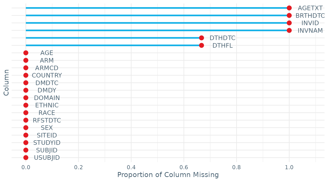
#> $studyid
#> # A tibble: 1 × 2
#>   STUDYID     n
#>   <chr>   <int>
#> 1 RPTESTB     3
#>
#> $sex
#>    SEX n
#> 1    F 2
#> 2    M 1
#> 3 <NA> 0
#>
#> $age
#> # A tibble: 1 × 7
#>   n_USUBJID AGE_min AGE_max n_missing_AGE n_AGE_under_6M n_AGE_under_18Y
#>       <int>   <dbl>   <dbl>         <int>          <int>           <int>
#> 1         3       4      67             0              0               1
#> # ℹ 1 more variable: n_AGE_over_90Y <int>
#>
#> $missingness
#> STUDYID  DOMAIN USUBJID  SUBJID RFSTDTC  DTHDTC   DTHFL  SITEID   INVID  INVNAM
#>   0.000   0.000   0.000   0.000   0.000   0.667   0.667   0.000   1.000   1.000
#> BRTHDTC     AGE  AGETXT     SEX    RACE  ETHNIC   ARMCD     ARM COUNTRY   DMDTC
#>   1.000   0.000   1.000   0.000   0.000   0.000   0.000   0.000   0.000   0.000
#>    DMDY
#>   0.000

check_data(LB_RPTESTB)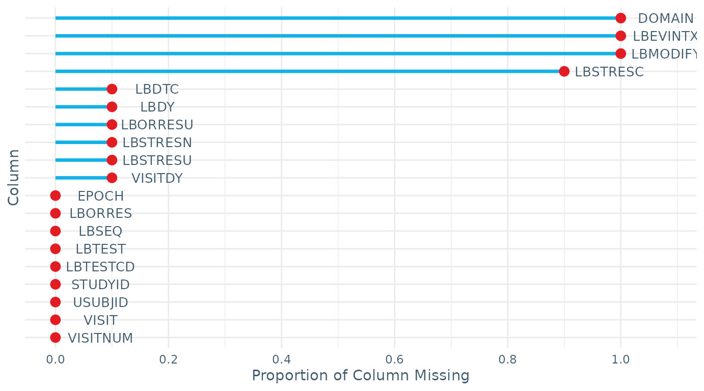
#> $studyid
#> # A tibble: 1 × 2
#>   STUDYID     n
#>   <chr>   <int>
#> 1 RPTESTB    10
#>
#> $testcd
#> # A tibble: 3 × 17
#>   STUDYID TESTCD   min    q5   q25   q50   q75   q95   max n_UNITS UNITS   n_LOC
#>   <chr>   <chr>  <dbl> <dbl> <dbl> <dbl> <dbl> <dbl> <dbl>   <int> <chr>   <int>
#> 1 RPTESTB HCG       NA  NA    NA    NA     NA    NA     NA       0 ""          0
#> 2 RPTESTB HGB       88  89.8  95.8  98.5  100.  102.   102       1 "g/L"       0
#> 3 RPTESTB PLAT      90  91    95   100    140.  173.   181       1 "10^9/…     0
#> # ℹ 5 more variables: LOC <chr>, n_METHOD <int>, METHOD <chr>, n_SPEC <int>,
#> #   SPEC <chr>
#>
#> $missingness
#>  STUDYID   DOMAIN  USUBJID    LBSEQ LBTESTCD   LBTEST  LBORRES LBMODIFY
#>      0.0      1.0      0.0      0.0      0.0      0.0      0.0      1.0
#> LBORRESU LBSTRESC LBSTRESN LBSTRESU VISITNUM    VISIT  VISITDY    EPOCH
#>      0.1      0.9      0.1      0.1      0.0      0.0      0.1      0.0
#>    LBDTC     LBDY LBEVINTX
#>      0.1      0.1      1.0
Miscellaneous Functions
table_variables() is a simple function to tabulate the
variables in a domain. Not all domains are currently covered in this
function but most are. This function may be useful when deciding which
variables to include in the prepare_domain() output.
table_variables(VS_RPTESTB, "vS")
#>
#>    BMI HEIGHT   TEMP WEIGHT
#>      3      3      9      3
convert_age_to_years() simplifies the AGE
and AGEU information to AGE_YEARS by
converting the various units (days, weeks, months) to years. This is
used within prepare_domain() and check_data()
(if age_in_years = FALSE)
age_df <- DM_RPTESTB %>% select(STUDYID, DOMAIN, USUBJID, AGE, AGEU)
age_df
#> # A tibble: 3 × 5
#>   STUDYID DOMAIN USUBJID       AGE AGEU
#>   <chr>   <chr>  <chr>       <dbl> <chr>
#> 1 RPTESTB DM     RPTESTB_001    67 YEARS
#> 2 RPTESTB DM     RPTESTB_002    18 YEARS
#> 3 RPTESTB DM     RPTESTB_003    48 MONTHS

convert_age_to_years(age_df)
#> # A tibble: 3 × 4
#>   STUDYID DOMAIN USUBJID     AGE_YEARS
#>   <chr>   <chr>  <chr>           <dbl>
#> 1 RPTESTB DM     RPTESTB_001        67
#> 2 RPTESTB DM     RPTESTB_002        18
#> 3 RPTESTB DM     RPTESTB_003         4